Build in models

PCA

Code

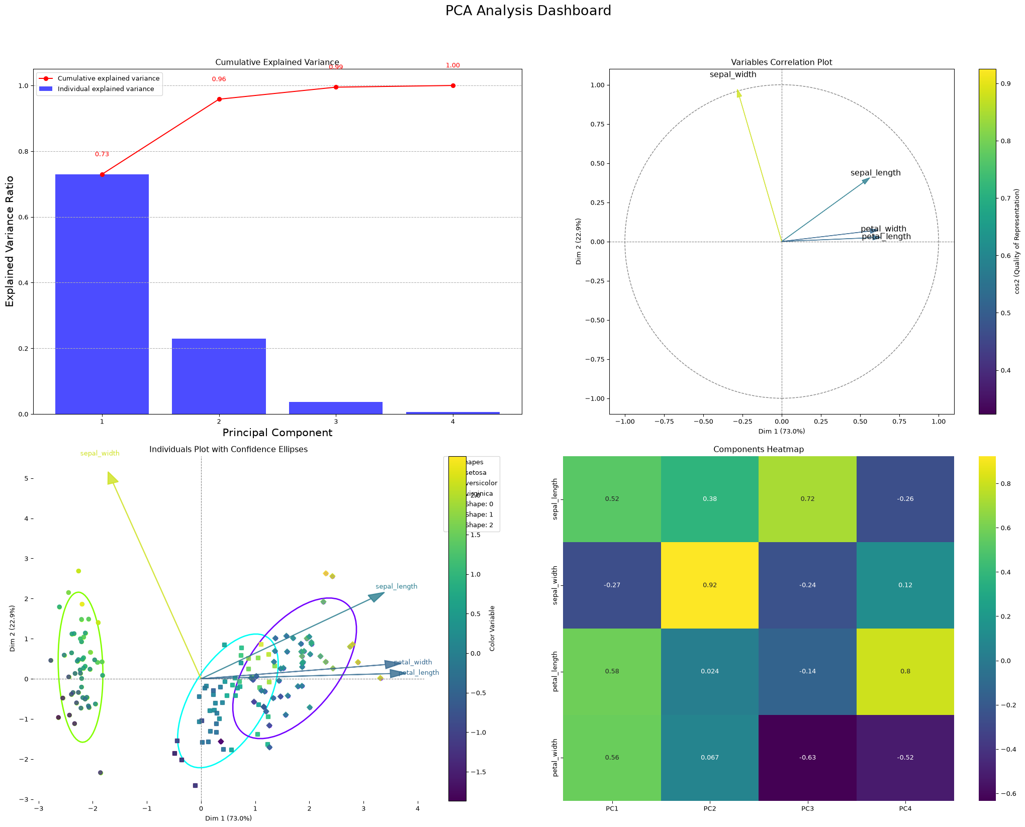
from BayesForge import bf
import jax.numpy as jnp

m= bf()
m.data(m.load.iris(only_path=True))
m.data_on_model = dict(
    X=jnp.array(m.df.iloc[:,0:-2].values)
)
m.fit(m.models.pca(type="classic"), progress_bar=False) # or robust, sparse, classic, sparse_robust_ard

_ = m.models.pca.plot(
    X=m.df.iloc[:,0:-2].values,
    y=m.df.iloc[:,-2].values, 
    feature_names=m.df.columns[0:-2], 
    target_names=m.df.iloc[:,-1].unique(),
    color_var=m.df.iloc[:,0].values,
    shape_var=m.df.iloc[:,-2].values
)

bf v 0.0.58 package loaded
jax.local_device_count 32

Survival analysis

Piecewise-constant (piecewise-exponential) hazard model. Time is cut into fixed intervals; import_time_even builds the per-interval death and exposure matrices, and censoring is handled by exposure dropping to 0 once a subject leaves the risk set.

Code

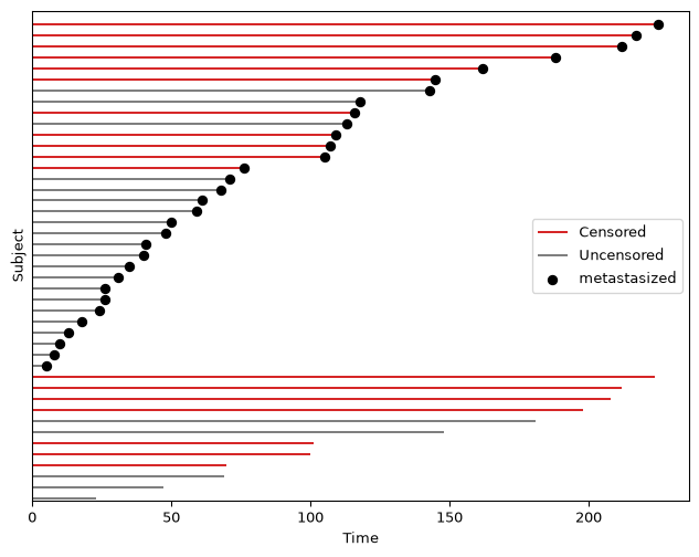
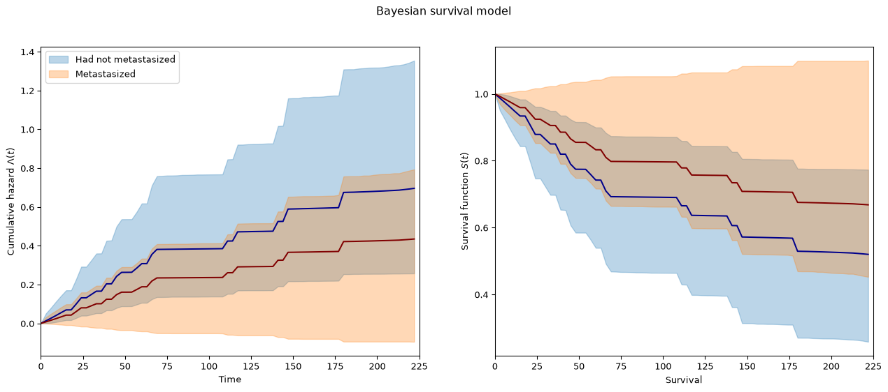
from BayesForge import bf
import jax.numpy as jnp

m = bf()
data_path = m.load.mastectomy(only_path=True)
m.data(data_path, sep=',')
m.df.metastasized = (m.df.metastasized.values == "yes").astype(jnp.int64)

# Discretise follow-up time into intervals and register the event indicator.
m.models.survival.import_time_even(
    m.df.time.values,
    m.df.event.values, interval_length=3
)

# Time-fixed (patient-level) covariates.
m.models.survival.import_covF(
    m.df.metastasized.values, ['metastasized']
)

# Time-varying covariates ⚠️ Experimental feature
# m.models.survival.import_covV

# Censoring plot: one line per subject (follow-up length), red = censored,
# grey = event observed, dot = metastasized.
m.models.survival.plot_censoring(cov='metastasized')

# Priors (shown with their defaults, override before fit):
#   Baseline_rate ~ Gamma(*baseline_rate_prior)  -> near-flat, one rate/interval
#   Hazard_rate_<cov> ~ Normal(0, hazard_rate_prior_scale)  -> log-hazard effect
m.models.survival.baseline_rate_prior = (0.01, 0.01)
m.models.survival.hazard_rate_prior_scale = 10.0

# 4 chains + target_accept_prob=0.99: the near-empty late baseline intervals
# make the geometry stiff, so a high acceptance target keeps mixing healthy.
m.fit(m.models.survival.model, num_samples=2000, num_warmup=2000,
      num_chains=4, target_accept_prob=0.99, progress_bar=False)

m.summary()

# Posterior cumulative hazard (left) and survival S(t)=exp(-Lambda(t)) (right)
# by covariate group. Effect size/direction: read beta (hazard ratio e^beta)
# from m.summary().
_ = m.models.survival.plot_surv(beta='Hazard_rate_metastasized')

jax.local_device_count 32
------------------------------------------------------------------------------
Survival concern 44 individuals in 76 intervals.
26.0 individuals experienced the event.
------------------------------------------------------------------------------
Covariates imported: ['metastasized']
Surv object now has 1 covariates: ['metastasized']
⚠️This function is still in development. Use it with caution. ⚠️
⚠️This function is still in development. Use it with caution. ⚠️
⚠️This function is still in development. Use it with caution. ⚠️
⚠️This function is still in development. Use it with caution. ⚠️
⚠️This function is still in development. Use it with caution. ⚠️
⚠️This function is still in development. Use it with caution. ⚠️
⚠️This function is still in development. Use it with caution. ⚠️
⚠️This function is still in development. Use it with caution. ⚠️

Gaussian Mixture Models

Code

from BayesForge import bf
from sklearn.datasets import make_blobs
m = bf()

# Generate synthetic data
data, true_labels = make_blobs(
    n_samples=500, centers=8, cluster_std=0.8,
    center_box=(-10,10), random_state=101
)

m.data_on_model = {"data": data, "K": 8}
m.fit(m.models.gmm, progress_bar=False)  # MCMC over the mixture parameters
_ = m.plot(X=data, sampler=m.sampler)    # ⚠️ Experimental feature

jax.local_device_count 32
⚠️This function is still in development. Use it with caution. ⚠️
⚠️This function is still in development. Use it with caution. ⚠️

Dirichlet Process Mixture Models

Code

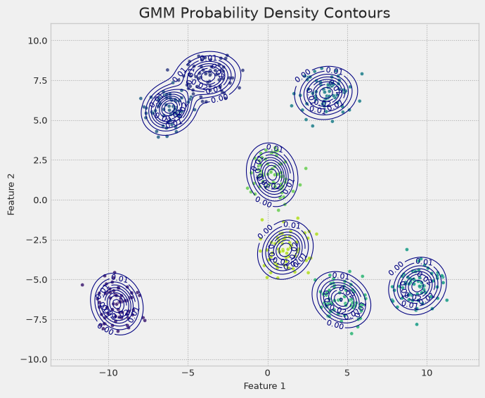
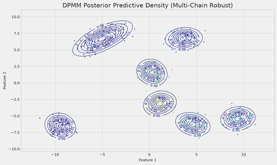
from BayesForge import bf
from sklearn.datasets import make_blobs
m = bf()

# Generate synthetic data
data, true_labels = make_blobs(
    n_samples=500, centers=8, cluster_std=0.8,
    center_box=(-10,10), random_state=101
)
# T = truncation level (max clusters). method='marginal' integrates out the
# cluster assignments (NUTS-friendly); 'latent' samples them explicitly.
# DPMM priors are already centred on the data mean/scale - no flag needed.
m.data_on_model = dict(data=data, T=10, method='marginal')
m.fit(m.models.dpmm, num_samples=500, num_warmup=500, num_chains=2,
      progress_bar=False)
_ = m.plot(data, m.sampler)

jax.local_device_count 32
Model found 7 clusters.
Computing density across all chains (this might take a moment)...

Network Models

Code

from BayesForge import bf
import jax.numpy as jnp

# Setup device------------------------------------------------
m = bf(platform='cpu')
# Simulate data ------------------------------------------------
N = 50
individual_predictor = m.dist.normal(0,1, shape = (N,1), sample = True)

kinship = m.dist.bernoulli(0.3, shape = (N,N), sample = True)
kinship = kinship.at[jnp.diag_indices(N)].set(0)

def sim_network(kinship, individual_predictor):
  # Intercept
  alpha = -8

  # SR
  sr = m.net.sender_receiver(individual_predictor, individual_predictor, s_mu = 0.4, r_mu = -0.4, sample = True)

  # D
  DR = m.net.dyadic_effect(kinship, d_sd= 1, sample = True)

  return m.dist.bernoulli(logits = alpha + sr + DR, sample = True)


network = sim_network(m.net.mat_to_edgl(kinship), individual_predictor)

m.net.viz(m.net.edgl_to_mat(network))

jax.local_device_count 32